Summary of the Project

Our project is similar to that of an “escape room,” where the agent must find an exit of a room within a reasonable amount of time. However, the agent must avoid death as there is a fire that spreads throughout the map and should aim to recover resources along the way. As a result, dying is equivalent to a penalty and recovering resources and finding exits within a short amount of time (or with minimal steps) is essential to rewards.

Approach

Aforementioned on our home page…: to start this project, we first created random maps by writing a program that helps us generate a map via XML strings. The user would input the size of the map he or she wants, and shortly after, the program will output a long string for the map. This map includes exit point(s), blocks/areas where the agent is not able to access, and a location for the fire to start spreading. It is important to note the material of the generated map. We decided to set the material of the floor to be carpet so that the fire can spread; however, in Minecraft, it is normal for the fire to go out after a certain period of time. To battle this, we put netherrack blocks below the carpet so that when the carpet burns out, the fire continues and never estinguishes. In order to have our fire spread in a somewhat ‘controlled path’ so that it does not spread everywhere, we used sea lanterns to prevent the fire from haphazardly spreading in any direction.

To avoid overfitting our agent on one kind of map, we used this program to generate random mazes for our agent to train and test. After the maze is built, we spawn the agent in a random location. The image below shows the final result of a randomly generated 5x5 sized maze.

_{Image 1 (Above): An example of our randomly generated maze with fire.}

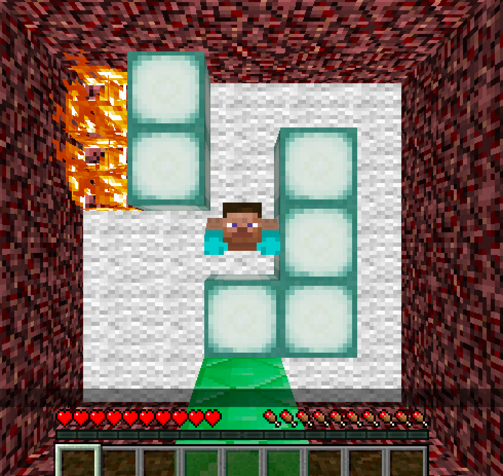
As of yet, we have not implemented any resources within the program.

For the artificial intelligence, we decided to use the Deep-Q Learning algorithm which uses greedy-epsilon based policy. Deep-Q Learning is based on the following:

_{Figure 1 (Above): Bellman Equation for Optimality1}

We used this formula in our algorithm and defined the variables as followed:

• S: the current state which is the grid observation (ie a birds eye view of the map). It includes the information of our maze and the surroundings relative to the agent. Alternatively, the agent is able to see its surroundings as 9x9 grid, where the agent is at the center of it
• S’: Next state after taking action A’
• A: the current action that our agent will take. Currently, our agent can make four moves [move north, move south, move east, move west]. As of yet, it cannot pick up resources as it aims to find the exit in a minimal number of steps.
• A’: the future action
• R: is our expected reward based on the action our agent takes.
• γ (gamma): Discount factor. We set our gamma = 0.99 as that is the staple norm in Q-learning.

We used Tensorflow to build our Neural Network, and our network consists of three convolutional layers, followed by 2 fully connected layers. The last fully connected layer outputs values from 0-3 which is mapped to our action space. As for our input to the network, we used a little trick. Malmo offers a feature to observe the surrounding blocks by tag in the mission XML file, and we get it from Malmo via a JSON file as a 2D array. We then convert that 2D array as a pixel representation of the grid and feed it to the Neural Network as a grayscale image.

The techniques we used for our DQN is the Experience Replay Memory and uses two separate networks: Q-network and Target Network.

• The Replay Memory consists of tuples of [ “state”, “action”, “reward”, “next_state”, “done”]. We then use the Replay Memory to sample a batch of size 32 to train our agent. Each step an agent takes is stored in the replay memory. In the beginning of training, we fill around 10% of the total replay memory with random exploration and gradually fills it as the agent trains. Once it is filled, the earliest memory is popped.

• The Target Network is used for calculating our loss and updates every N number of episodes. For our loss value, we use the squared differences of the Q-network and Target Network and performed gradient descent on it.

_{Figure 2 (Above): Loss Function2}

To evaluate our progress, we used one of Tensorflow features, Tensorboard, to display the metrics. With the help of Tensorflow and Tensorboard in our approach, we were able to obtain a graphical model of our data and its trends to ensure that our agent is working properly such that it fulfills our sanity case - that our agent does not constantly die in the fire.

Another big part of our project is generating a random maze. The user can choose their maze size and generate a random maze XML file. In order to avoid our agent from overfitting to only one map, we incorporated multiple random mazes into our training process. Every 20 episodes, we randomly choose from one of our randomly generated mazes and train the agent on that map. Even during Experience Replay Memory initialization, every 20 step, we change the maze. Doing this increases our training time and makes it harder for the agent to learn, but prevents the agent from overfitting to one specific map and help our agent to perform well on unseen test map.

Evaluation

As an overview, we decided on the following factors for our analysis:

Baseline:

Our previous baseline is so that the agent does not die in the fire and is able to find the exit. However, for this status report, our baseline changed such that the a random agent can perform random movements until it either dies to the spreading fire or exits the maze by luck.

Quantitative Analysis for Status Report:

The number of steps taken to find the exit. Ideally, we would want the number of steps to have a general decreasing trend on a graph. During the training process, we should see an increase in the reward. It indicates that agent is solving the maze quicker each time, since there is a penalty for each extra move the agent makes.

Qualitative Analysis for Status Report:

The agent does not run into the fire and die; alternatively, the agent is able to escape the fire, should it run into it.

The following graphs represent our current progress on the algorithm and agent’s performance.

_{Graph 1 (Above): Episode Length. It shows the general trend of our episode lengths throughout the training.}

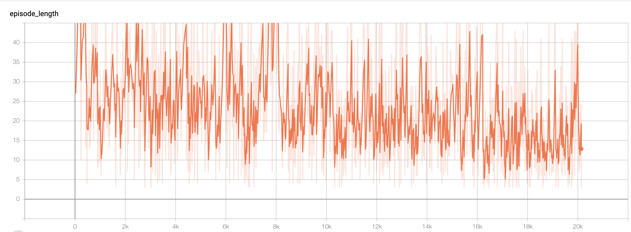
Graph 1 demonstrates our overall trend on the episode length. Specifically, it is measured through the number of steps, or, rather, actions taken by the agent. Overall, it took a total of 20,000 steps during training and the general trend of the episode length decreases throughout the graph. This trend is supported in our following graphs of the episode reward, epsilon, loss per steps (i.e., error rate), and the max Q-value.

_{Graph 2 (Above): Episode Reward. The general trend in the reward.}

_{Graph 3 (Above): Epsilon. The overall change of our epsilon value (eg chance of random action).}

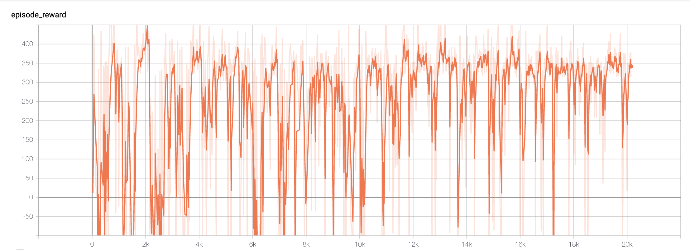
With our episode reward graph (i.e., Graph 2), we measure how much our agent is rewarded based on the actions it takes and whether it reaches the goal or mission ends prematurely, i.e., run out of time or burned to death.

The following displays our reward system:

• Reaching a goal, in our case touching an emerald block: +100
• Touching a fire: -55
• Touching inner maze wall: -20
• Dying: -10
• Making a move: -1

We want our agent to have its reward increasing to show that it is learning throughout its training sessions. Thus, the episode reward is relative to the number of steps the agent has taken. We estimate our graph to have numerous downward spikes due to our epsilon value - where our agent takes a random action as a way to explore the maze or its environment and avoid suboptimal convergence. However, throughout the entire graph, we can see that it gradually converges and stabilizes as epsilon decreases as seen in Graph 3.

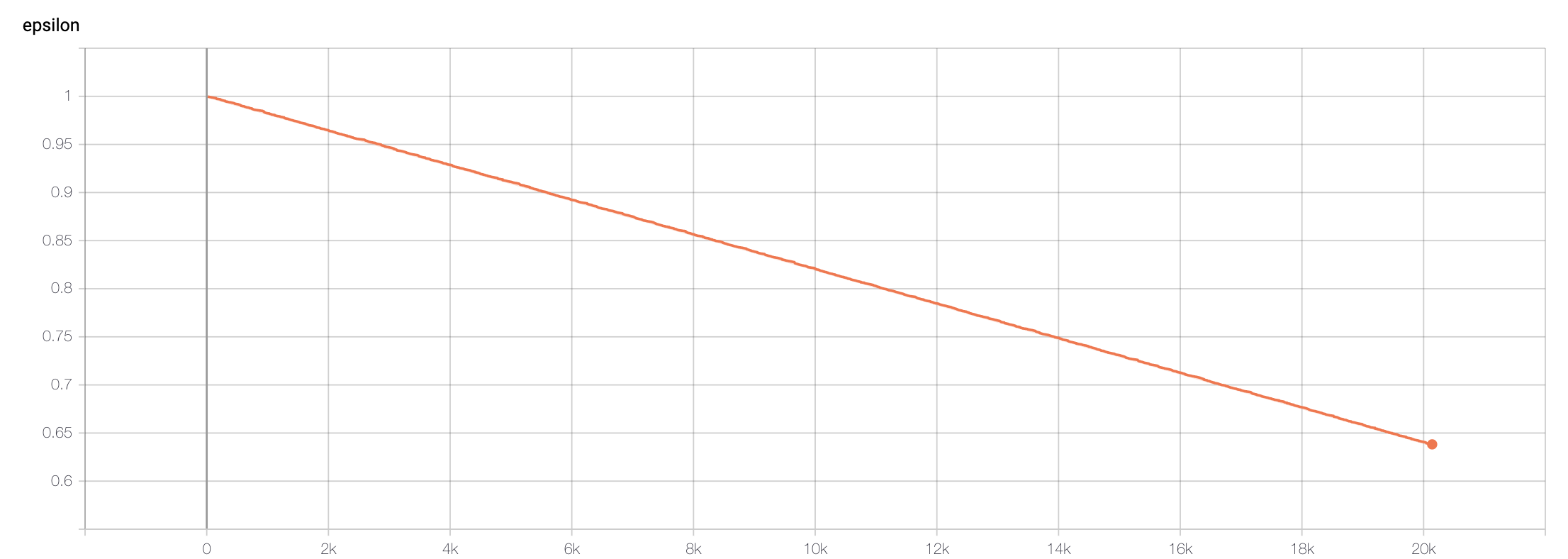
The general trend with epsilon starts at 1, and in Deep-Q learning, we should aim for epsilon to decrease to 0.1 such that the agent no longer or seldom takes random actions. At 20,000 steps (as corresponding to our episode reward and episode length graph), our epsilon has decreased to 0.63. Ideally, if more training were done with a greater number of steps taken (eg as we reach ~50,000 steps), we would be able to see epsilon closer to the value 0.1.

_{Graph 4 (Above): Loss. This graph shows our general loss throughout training.}

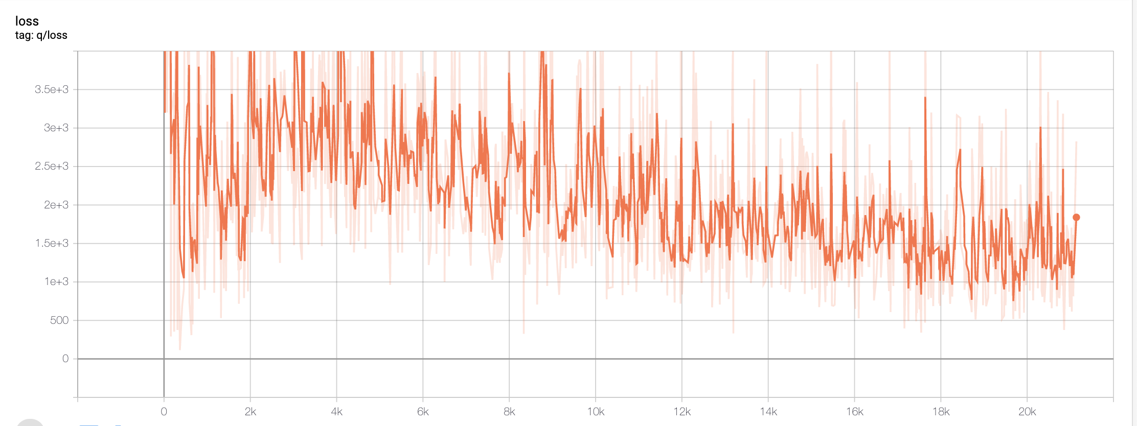
In machine learning, we aim to minimize our loss, or rather, the error rate as we train our agent. With Deep Q-learning, the agent should predict a move and its reward and select the action that will provide it with the highest reward. To ensure that our agent was minimizing its losses, we graphed the overall trend of our agent in respect to its error rate (Graph 4). We can see here that the error gradually decreases in respect to the number of steps our agent has taken. This finally leads us to our overall maximum Q-value trend.

_{Graph 5 (Above): Max Q-Value. The graph that shows an increasing trend in the maximum Q-value.}

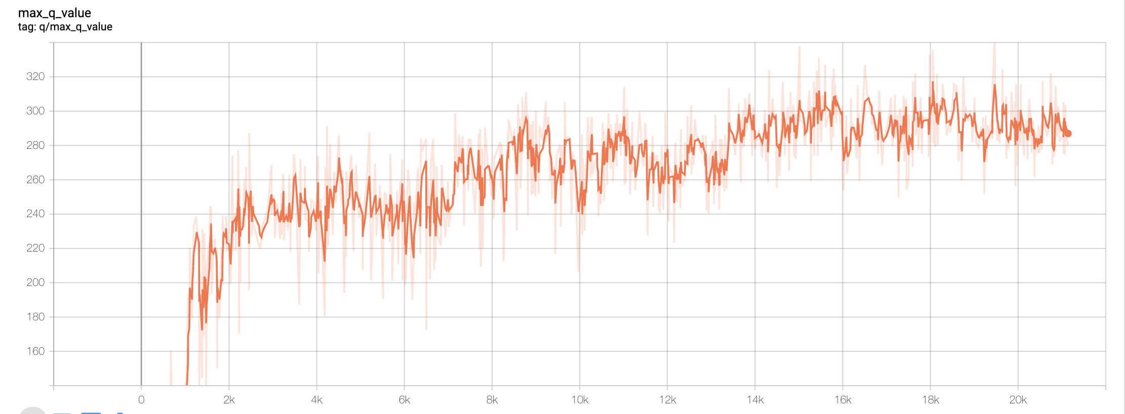
Overall, our maximum Q-value increases which denotes a higher trend in performance in respect to the number of total steps taken. Our goal is to maximize the Q-value so that it helps the agent predict the next best action based on the expected reward. With a higher Q-value, it can thus choose the next best action and thereby minimizing loss.

We trained our agent for approximately 3 hours and 40 minutes. It is important to note, however, that the fire acts and spreads randomly and is beyond our control in terms of its speed and direction(s) when the fire is not blocked by a sea lantern. Consequently, this made it extremely difficult to train the agent so that the agent can dodge the fire. On bigger maps, it would take longer (i.e, days of training) and a larger neural network.

Remaining Goals and Challenges

Currently, our agent works in a 5x5 environment. Originally, we had planned a 10x10 environment shown below but realized that after a number of training episodes, our agent became ‘dumber’ and was performing worse as time went on (eg taking a longer time to find the exit, dying in the fire more, etc). After consulting with the Professor and TA, we realized that in order for our agent to work in a larger environment, more complicated factors need to be considered (eg better policy-based learning in our neural network as opposed to a greedy-epsilon policy). Since this became a road block part way through our project, we decided to settle for a smaller 5x5 map, rather than our 10x10 map, to ensure our agent is working correctly. In the coming weeks, we hope to get our agent to work on 10x10 maps and/or maps that are larger than 5x5.

In addition, we aim to have resources (e.g., food in Minecraft) implemented for our agent to collect. As of now, we are focusing on ensuring that our agent learns properly in the given environment.

Video

Resources Used

[1], [2]. Matiisen, Tambet. “Guest Post (Part I): Demystifying Deep Reinforcement Learning.” Intel AI, Intel. Date Published on 22 December 2015. URL. https://www.intel.ai/demystifying-deep-reinforcement-learning/#gs.eggq2z

Britz, Denny. Reinforcement Learning.(2019). GitHub Repository. https://github.com/dennybritz/reinforcement-learning/tree/master/DQN

Juliani, Arthur. “Simple Reinforcement Learning with Tensorflow Part 4: Deep Q-Networks and Beyond.” Medium, Medium, Date Published on 2 September 2016. URL. https://medium.com/@awjuliani/simple-reinforcement-learning-with-tensorflow-part-4-deep-q-networks-and-beyond-8438a3e2b8df

Tabular_learning.py tutorial, included in Malmo